Learning ggtree
You can’t even begin to understand biology, you can’t understand life, unless you understand what it’s all there for, how it arose - and that means evolution. — Richard Dawkins
Introduction
ggtree is a bioconductor package which facilitates the implements for viewing, annotating and manipulating phylogenetic trees.
In addition to Newick and Nexus, ggtree supports the file formats using these parser functions:
read.beastfor parsing output of BEASEread.codemlfor parsing output of CODEML (rstandmlcfiles)read.codeml_mlcfor parsingmlcfile (output ofCODEML)read.hyphyfor parsing output of HYPHYread.jplacefor parsingjplacefile including output from EPA and pplacerread.nhxfor parsingNHXfile including output from PHYLODOG and RevBayesread.paml_rstfor parsingrstfile (output ofBASEMLandCODEML)read.r8sfor parsing output of r8sread.raxmlfor parsing output of RAxML
Here is an overview of all tree object: 
Simple Tour
Some Basic Functions: - ggtree(tree_object): Viewing a phylogenetic tree - get.fields: get the annotation features - get.tree: onvert tree object to phylo (or multiPhylo for r8s) object - groupOTU: clustering related OTUs (from tips to their most recent common ancestor),monophyletic (clade), polyphyletic or paraphyletic - fortify: convert tree object to a data.frame
Annatation geometry objects: + geom_text for displaying the node (if available) and tip labels simultaneously + geom_tiplab for adding tip labels + geom_cladelabel for labelling selected clades + geom_hilight for highlighting selected clades + geom_range to indicate uncertainty of branch lengths + geom_strip for adding strip/bar to label associated taxa (with optional label) + geom_taxalink for connecting related taxa + geom_treescale for adding a legend of tree scale
ggtree provides write.jplace function to combine Newick tree file and user’s own data to a single jplace file that can be parsed and the data can be used to annotate the tree directly in ggtree.
library("ape") library("Biostrings") library("ggplot2") library("ggtree") |
OK, let’s read the phylogenetic gree(i.e. beast tree).
file <- system.file("extdata/BEAST", "beast_mcc.tree", package="treeio") beast <- read.beast(file) beast |
## 'beast' S4 object that stored information of ## 'D:/Program Files/R-3.4.4/library/treeio/extdata/BEAST/beast_mcc.tree'. ## ## ...@ tree: ## Phylogenetic tree with 15 tips and 14 internal nodes. ## ## Tip labels: ## A_1995, B_1996, C_1995, D_1987, E_1996, F_1997, ... ## ## Rooted; includes branch lengths. ## ## with the following features available: ## 'height', 'height_0.95_HPD', 'height_median', 'height_range', 'length', ## 'length_0.95_HPD', 'length_median', 'length_range', 'posterior', 'rate', ## 'rate_0.95_HPD', 'rate_median', 'rate_range'. |
# Tips: length_95%_HPD will be changed to length_0.95_HPD |
So, we must intensely curious about what the beast looks like in the simplest ggtree function, the grammar of graphics on the tree, just simply tap the ggtree(beast), and ggtree, is a short cut to visualize a tree which equal to ggplot(beast, aes(x, y)) + geom_tree() + theme_tree(). By default, the tree is viewed in ladderize form, set the parameter ladderize = FALSE to disable it.
The branch.length is used to scale the edge, defulat is phylogram, set the parameter branch.length = "none" to only view the tree topology (cladogram)
multiplot(ggtree(beast),ggtree(beast, ladderize=FALSE),ggtree(beast, branch.length = "none"),ncol=3,labels = LETTERS[1:3]) |

geom_treescale() supports the following parameters: + x and y for tree scale position + width for the length of the tree scale + fontsize for the size of the text + linesize for the size of the line + offset for relative position of the line and the text + color for color of the tree scale
ggtree(beast)+geom_treescale(x=0, y=12, width=6, color='red',fontsize=8, linesize=2, offset=-1) |

ggtree supports several layouts, including - rectangular(by default) - slanted - circular - fan - unrooted for Phylogram and Cladogram, unrooted , layout, time-scaled and two dimentional phylogenies.
# Phylogram # Bg aded multiplot(ggtree(beast, layout="slanted") + theme_tree("aliceblue"),ggtree(beast,layout="circular")+ theme_tree("azure"),ggtree(beast, layout="fan",open.angle=180) + theme_tree("beige"),ncol=3) |

# Cladogram # Labels added multiplot(ggtree(beast, layout="slanted",branch.length='none') + geom_tiplab(aes(x=branch), size=3, color="purple", vjust=-0.3,hjust=0.3) ,ggtree(beast,layout="circular",branch.length='none') + geom_tiplab(aes(angle=angle),size=3, color='blue'),ggtree(beast, layout="fan",open.angle=180,branch.length='none') + geom_tiplab2(color='blue',size=3),ncol=3) |

And Using geom_range layer to display uncertainty of branch length.
ggtree(beast) + geom_range(range='length_0.95_HPD', color='magenta', alpha=.8, size=1.5) |
 Moreover,the
 heigh_0.95_HPD is meaningful since the branch is scaled by height(default, check using get.fields, it is the order of [‘height’,‘length’,‘rate’]). We can redefine the branch by specifing branch.length in ggtree function.
ggtree(beast, branch.length = 'rate') + geom_range(range='rate_0.95_HPD', color='cyan', alpha=.8, size=1.5) + ggtitle("Substitution rate") + theme_tree2() |

# #== # ggtree(rescale_tree(beast, branch.length = 'rate')) + geom_range(range='rate_0.95_HPD', color='cyan', alpha=.8, size=1.5) + ggtitle("Substitution rate") + theme_tree2() |
Color Tree
ggtree(beast, aes(color=rate)) + scale_color_continuous(low='darkgreen', high='red') + theme(legend.position="right") |

But, the simplicity of this the tree plot is in the raw, how about slightly making up for better visualization.
Note: Showing all the internal nodes and tips in the tree can be done by adding a layer of points using geom_nodepoint, geom_tippoint or geom_point.
# HPD:highest posterior density ggtree(beast, ndigits=1, branch.length = 'none', color="firebrick", size=1, linetype="dotted") + geom_text(aes(x=branch, label=length_0.95_HPD), vjust=-.5, color='darkgray') + geom_point(aes(shape=isTip, color=isTip), size=3) + ggtitle(" Phylogentic Tree") |
## Warning: Removed 1 rows containing missing values (geom_text). |

# OR ggtree(beast, ndigits=1, branch.length = 'none', color="firebrick", size=1, linetype="dotted") + geom_text(aes(x=branch, label=length_0.95_HPD), vjust=-.5, color='darkgray') + geom_nodepoint(color="#b5e521", alpha=1/4, size=10) + geom_tippoint(color="#FDAC4F", shape=8, size=3) + ggtitle(" Phylogentic Tree") |
## Warning: Removed 1 rows containing missing values (geom_text). |

Finally lets convert ggtree object to our favourite data.frame in R.
beast_data <- fortify(beast) # only show 10 colums coz the table was too enormous knitr::kable(head(beast_data[,1:10], 10)) |
| node | parent | branch.length | x | y | label | isTip | branch | angle | height |
|---|---|---|---|---|---|---|---|---|---|
| 1 | 26 | 1.3203366 | 19.926089 | 13 | A_1995 | TRUE | 19.265920 | 312 | 18 |
| 2 | 25 | 3.2619545 | 20.926089 | 12 | B_1996 | TRUE | 19.295111 | 288 | 17 |
| 3 | 28 | 3.3119924 | 19.926089 | 7 | C_1995 | TRUE | 18.270092 | 168 | 18 |
| 4 | 17 | 8.8216633 | 11.926089 | 1 | D_1987 | TRUE | 7.515257 | 24 | 26 |
| 5 | 29 | 3.2710481 | 20.926089 | 9 | E_1996 | TRUE | 19.290565 | 216 | 17 |
| 6 | 27 | 0.8311578 | 21.926089 | 14 | F_1997 | TRUE | 21.510510 | 336 | 16 |
| 7 | 21 | 5.1939723 | 16.926089 | 6 | G_1992 | TRUE | 14.329102 | 144 | 21 |
| 8 | 23 | 2.1125745 | 16.926089 | 10 | H_1992 | TRUE | 15.869801 | 240 | 21 |
| 9 | 24 | 1.7572880 | 18.926089 | 11 | I_1994 | TRUE | 18.047445 | 264 | 19 |
| 10 | 20 | 1.5614320 | 7.926089 | 5 | J_1983 | TRUE | 7.145373 | 120 | 30 |
Tree import
nwk & nhx file
nwk <- system.file("extdata", "sample.nwk", package="treeio") tree <- read.tree(nwk) p <- ggtree(tree) + geom_tippoint(color="steelblue", alpha=1/4, size=10) p |

# %<% for update tree # rtree for Generating Random Trees p %<% rtree(30) |

nhxfile <- system.file("extdata/NHX", "ADH.nhx", package="treeio") nhx <- read.nhx(nhxfile) ggtree(nhx) + geom_tiplab() + geom_point(aes(color=S), size=5, alpha=.5) + theme(legend.position="right") + geom_text(aes(x=branch,label=branch.length), vjust=-.5) |
## Warning: Removed 1 rows containing missing values (geom_text). |

Phylip file
phyfile <- system.file("extdata", "sample.phy", package="treeio") phylip <- read.phylip(phyfile) phylip |
## 'phylip' S4 object that stored information of ## 'D:/Program Files/R-3.4.4/library/treeio/extdata/sample.phy'. ## ## ...@ tree: ## Phylogenetic tree with 15 tips and 13 internal nodes. ## ## Tip labels: ## K, N, D, L, J, G, ... ## ## Unrooted; no branch lengths. ## ## with sequence alignment available (15 sequences of length 2148) |
User can view sequence alignment with the tree via msaplot() function.
msaplot(phylip, offset=1) |
 ### jplace file
jpf <- system.file("extdata/sample.jplace", package="treeio") jp <- read.jplace(jpf) print(jp) |
## 'jplace' S4 object that stored information of ## 'D:/Program Files/R-3.4.4/library/treeio/extdata/sample.jplace'. ## ## ...@ tree: ## Phylogenetic tree with 13 tips and 12 internal nodes. ## ## Tip labels: ## A, B, C, D, E, F, ... ## ## Rooted; includes branch lengths. ## ## with the following features available: ## 'edge_num', 'likelihood', 'like_weight_ratio', 'distal_length', ## 'pendant_length'. |
# get.placements method to access the placement ## get only best hit get.placements(jp, by="best") |
## name edge_num likelihood like_weight_ratio distal_length pendant_length ## 1 AA 24 -61371.30 0.333344 3e-06 0.003887 ## 2 BB 1 -61312.21 0.333335 1e-06 0.000003 ## 3 CC 8 -61312.23 0.200011 1e-06 0.000003 |
## get all placement get.placements(jp, by="all") |
## name edge_num likelihood like_weight_ratio distal_length pendant_length ## 1 AA 24 -61371.30 0.333344 0.000003 0.003887 ## 2 BB 1 -61312.21 0.333335 0.000001 0.000003 ## 3 BB 2 -61322.21 0.333322 0.000003 0.000003 ## 4 BB 550 -61352.21 0.333322 0.000961 0.000003 ## 5 CC 8 -61312.23 0.200011 0.000001 0.000003 ## 6 CC 9 -61322.23 0.200000 0.000003 0.000003 ## 7 CC 10 -61342.23 0.199992 0.000003 0.000003 |
rst and mlc file (PAML)
Softwares using rst: - BASEML : each ten bases are separated by one space - CODEML : each three bases (triplet) are separated by one space
## from BASEML brstfile <- system.file("extdata/PAML_Baseml", "rst", package="treeio") brst <- read.paml_rst(brstfile) brst |
## 'paml_rst' S4 object that stored information of ## 'D:/Program Files/R-3.4.4/library/treeio/extdata/PAML_Baseml/rst'. ## ## ...@ tree: ## Phylogenetic tree with 15 tips and 13 internal nodes. ## ## Tip labels: ## A, B, C, D, E, F, ... ## Node labels: ## 16, 17, 18, 19, 20, 21, ... ## ## Unrooted; includes branch lengths. ## ## with the following features available: ## 'marginal_subs', 'joint_subs', 'marginal_AA_subs', 'joint_AA_subs'. |
## from CODEML crstfile <- system.file("extdata/PAML_Codeml", "rst", package="treeio") crst <- read.paml_rst(crstfile) crst |
## 'paml_rst' S4 object that stored information of ## 'D:/Program Files/R-3.4.4/library/treeio/extdata/PAML_Codeml/rst'. ## ## ...@ tree: ## Phylogenetic tree with 15 tips and 13 internal nodes. ## ## Tip labels: ## A, B, C, D, E, F, ... ## Node labels: ## 16, 17, 18, 19, 20, 21, ... ## ## Unrooted; includes branch lengths. ## ## with the following features available: ## 'marginal_subs', 'joint_subs', 'marginal_AA_subs', 'joint_AA_subs'. |
# use theme_tree2() to display the tree scale by adding x axis p <- ggtree(brst) + geom_text(aes(x=branch, label=marginal_AA_subs), vjust=-.5, color='brown') + theme_tree2() p |

The mlc file output by CODEML contains dN/dS estimation.
Note : / and * are not valid characters in names, they were changed to _vs_ and _x_ respectively.
So dN_vs_dS is dN/dS, N_x_dN is N*dN, and S_x_dS is S*dS.
mlcfile <- system.file("extdata/PAML_Codeml", "mlc", package="treeio") mlc <- read.codeml_mlc(mlcfile) mlc |
## 'codeml_mlc' S4 object that stored information of ## 'D:/Program Files/R-3.4.4/library/treeio/extdata/PAML_Codeml/mlc'. ## ## ...@ tree: ## Phylogenetic tree with 15 tips and 13 internal nodes. ## ## Tip labels: ## A, B, C, D, E, F, ... ## Node labels: ## 16, 17, 18, 19, 20, 21, ... ## ## Unrooted; includes branch lengths. ## ## with the following features available: ## 't', 'N', 'S', 'dN_vs_dS', 'dN', 'dS', 'N_x_dN', 'S_x_dS'. |
ggtree(mlc, branch.length = "dN_vs_dS", aes(color=dN_vs_dS)) + scale_color_continuous(name='dN/dS', limits=c(0, 1.5), oob=scales::squish, low="darkgreen", high="red")+ theme_tree2(legend.position=c(.9, .5)) |

Then, Combine them using read.codeml which is highly recommended, we can annotate dN/dS with the tree in rstfile and amino acid substitutions with the tree in mlcfile.
ml <- read.codeml(crstfile, mlcfile) ml |
## 'codeml' S4 object that stored information of ## 'D:/Program Files/R-3.4.4/library/treeio/extdata/PAML_Codeml/rst' and ## 'D:/Program Files/R-3.4.4/library/treeio/extdata/PAML_Codeml/mlc'. ## ## ...@ tree: ## Phylogenetic tree with 15 tips and 13 internal nodes. ## ## Tip labels: ## A, B, C, D, E, F, ... ## Node labels: ## 16, 17, 18, 19, 20, 21, ... ## ## Unrooted; includes branch lengths. ## ## with the following features available: ## 'marginal_subs', 'joint_subs', 'marginal_AA_subs', 'joint_AA_subs', 't', ## 'N', 'S', 'dN_vs_dS', 'dN', 'dS', 'N_x_dN', 'S_x_dS'. |
HYPHY tree
nwk <- system.file("extdata/HYPHY", "labelledtree.tree", package="treeio") ancseq <- system.file("extdata/HYPHY", "ancseq.nex", package="treeio") tipfas <- system.file("extdata", "pa.fas", package="treeio") hy <- read.hyphy(nwk, ancseq, tipfas) hy |
## 'hyphy' S4 object that stored information of ## 'D:/Program Files/R-3.4.4/library/treeio/extdata/HYPHY/labelledtree.tree', ## 'D:/Program Files/R-3.4.4/library/treeio/extdata/HYPHY/ancseq.nex' and ## 'D:/Program Files/R-3.4.4/library/treeio/extdata/pa.fas'. ## ## ...@ tree: ## Phylogenetic tree with 15 tips and 13 internal nodes. ## ## Tip labels: ## K, N, D, L, J, G, ... ## Node labels: ## Node1, Node2, Node3, Node4, Node5, Node12, ... ## ## Unrooted; includes branch lengths. ## ## with the following features available: ## 'subs', 'AA_subs'. |
ggtree(hy) + geom_text(aes(x=branch, label=AA_subs), vjust=-.5) |
 ### r8s file r8s output contains 3 trees, namely
 TREE, RATO and PHYLO for time tree, rate tree and absolute substitution tree respectively. Of Course, This is a time-scaled tree by specifying the parameter, mrsd (most recent sampling date).
r8s <- read.r8s(system.file("extdata/r8s", "H3_r8s_output.log", package="treeio")) ggtree(r8s, branch.length="TREE", mrsd="2014-01-01") + theme_tree2() + ggtitle("Divergence time") |

View 3 trees simultaneously.
# get.tree(r8s) # 3 phylogenetic trees ggtree(get.tree(r8s), aes(color=.id)) + facet_wrap(~.id, scales="free_x") |
 ### RAxML bootstraping analysis
raxml_file <- system.file("extdata/RAxML", "RAxML_bipartitionsBranchLabels.H3", package="treeio") raxml <- read.raxml(raxml_file) ggtree(raxml) + geom_label(aes(label=bootstrap, fill=bootstrap)) + geom_tiplab() + scale_fill_continuous(low='darkgreen', high='red') + theme_tree2(legend.position='right') |
 ### Merging tree Using
 tree <- merge_tree(tree_object_1, tree_object_2) %>% merge_tree(tree_object_3) %>% merge_tree(tree_object_4)
beast_file <- system.file("examples/MCC_FluA_H3.tree", package="ggtree") beast_tree <- read.beast(beast_file) rst_file <- system.file("examples/rst", package="ggtree") mlc_file <- system.file("examples/mlc", package="ggtree") codeml_tree <- read.codeml(rst_file, mlc_file) merged_tree <- merge_tree(beast_tree, codeml_tree) merged_tree |
## 'beast' S4 object that stored information of ## 'D:/Program Files/R-3.4.4/library/ggtree/examples/MCC_FluA_H3.tree'. ## ## ...@ tree: ## Phylogenetic tree with 76 tips and 75 internal nodes. ## ## Tip labels: ## A/Hokkaido/30-1-a/2013, A/New_York/334/2004, A/New_York/463/2005, A/New_York/452/1999, A/New_York/238/2005, A/New_York/523/1998, ... ## ## Rooted; includes branch lengths. ## ## with the following features available: ## 'height', 'height_0.95_HPD', 'height_median', 'height_range', 'length', ## 'length_0.95_HPD', 'length_median', 'length_range', 'posterior', 'rate', ## 'rate_0.95_HPD', 'rate_median', 'rate_range', 't', 'N', 'S', 'dN_vs_dS', ## 'dN', 'dS', 'N_x_dN', 'S_x_dS', 'marginal_subs', 'joint_subs', ## 'marginal_AA_subs', 'joint_AA_subs'. |
Now, we can use dN/dS inferred by CodeML to color the tree and annotate the tree with posterior inferred by BEAST.
ggtree(merged_tree, aes(color=dN_vs_dS), mrsd="2013-01-01", ndigits = 3) + geom_text(aes(label=posterior), vjust=.1, hjust=-.1, size=5, color="black") + scale_color_continuous(name='dN/dS', limits=c(0, 1.5), oob=scales::squish, low="green", high="red")+ theme_tree2(legend.position="right") |
 ### Specified file
The data contains amino acid substitutions from parent node to child node and GC contents of each node.
tree <- system.file("extdata", "pa.nwk", package="treeio") data <- read.csv(system.file("extdata", "pa_subs.csv", package="treeio"), stringsAsFactor=FALSE) print(tree) |
## [1] "D:/Program Files/R-3.4.4/library/treeio/extdata/pa.nwk" |
knitr::kable(head(data)) |
| label | subs | gc |
|---|---|---|
| A | R262K/K603R | 0.444 |
| B | R262K | 0.442 |
| C | N272S/I354T | 0.439 |
| D | K104R/F105L/E382D/F480S/I596T | 0.449 |
| E | T208S/V379I/K609R | 0.443 |
| F | S277P/L549I | 0.444 |
ggtree |
provides a function, _`write.jp | lace_, to combine a tree and an associated data and store them to a single _jplace`_ file. |
outfile <- tempfile() write.jplace(tree, data, outfile) jp <- read.jplace(outfile) print(jp) |
## 'jplace' S4 object that stored information of ## 'C:\Users\Lyole\AppData\Local\Temp\RtmpSK5Q4y\filef383a435e41'. ## ## ...@ tree: ## Phylogenetic tree with 15 tips and 13 internal nodes. ## ## Tip labels: ## K, N, D, L, J, G, ... ## ## Unrooted; includes branch lengths. ## ## with the following features available: ## 'label', 'subs', 'gc'. |
Tree Manipulation
ggtree implement several functions to manipulate a phylogenetic tree.
- taxa can be clustered together using
groupCladeorgroupOTUfunctions - clades can be collapsed via
collapsefunction - collapsed clade can be expanded by using
expandfunction - clade can be re-scale to zoom in or zoom out by
scaleCladefunction - selected clade can be rotated by 180 degree using
rotatefunction - position of two selected clades (should share a same parent) can be exchanged by
flipfunction
Node Manipulation
Get the internal node number using geom_text2 or get the internal node number by using MRCA()(most recent commond ancestor ) function, using viewClade to visualize a clade of a phylogenetic tree
And groupClade and groupOTU methods were designed for clustering clades or related OTUs. groupClade accepts an internal node or a vector of internal nodes to cluster clade/clades.
nwk <- system.file("extdata", "sample.nwk", package="treeio") tree <- read.tree(nwk) p <- ggtree(tree) + geom_text2(aes(subset=!isTip, label=node), hjust=-.3) + geom_tiplab() multiplot(p, ggtree(tree) %>% groupClade(node=21) + aes(color=group, linetype=group), viewClade(p, node=21),ncol=3) |

# MRCA(tree, tip=c('A', 'E')) # # 17 gzoom(p, grep("[HFG]", tree$tip.label)) |

tree <- groupClade(tree, node=c(21, 17)) multiplot(ggtree(tree, aes(color=group, linetype=group)) + geom_tiplab(aes(subset=(group==1))),ggtree(tree, aes(color=group, linetype=group)) + geom_tiplab(aes(subset=(group==2))),ncol=2) |

groupOTU accepts a vector of OTUs (taxa name) or a list of OTUs, related OTUs are not necessarily within a clade, they can be monophyletic (clade), polyphyletic or paraphyletic.
tree <- groupOTU(tree, c("D","E","F","G")) ggtree(tree, aes(color=group)) + geom_tiplab() |

tree2 <- groupOTU(ggtree(tree), LETTERS[4:7]) tree2 + aes(color=group) + geom_tiplab() + scale_color_manual(values=c("black", "firebrick")) |

cls <- list(c1=c("A", "B", "C", "D", "E"), c2=c("F", "G", "H"), c3=c("L", "K", "I", "J"), c4="M") tree <- groupOTU(tree, cls) library("colorspace") ggtree(tree, aes(color=group, linetype=group)) + geom_tiplab() + scale_color_manual(values=c("black", rainbow_hcl(4))) + theme(legend.position="right") |
 ### Clade Manipulation
expand & collapsed clade
p1 <- ggtree(tree) + geom_text2(aes(subset=!isTip, label=node), hjust=-.3) p2 <- collapse(p1, 21) + geom_point2(aes(subset=(node==21)), size=5, shape=23, fill="blue") p3 <- collapse(p2, 17) + geom_point2(aes(subset=(node==17)), size=5, shape=23, fill="red") p4 <- expand(p3, 17) p5 <- expand(p4, 21) multiplot(p1, p2, p3, p4, p5, ncol=5) |
 scale clade
multiplot(p1 + geom_hilight(21, fill = "GoldenRod") + geom_hilight(17, fill="forestGreen",alpha = 0.5), p1 %>% scaleClade(21, scale=0.3) %>% scaleClade(17, scale=0.5) + geom_hilight(21, fill="GoldenRod") + geom_hilight(17, fill="forestGreen"),ncol=2) |
 rotate clade
tree <- groupClade(tree, c(21, 17)) p <- ggtree(tree, aes(color=group)) + scale_color_manual(values=c("black", "firebrick", "steelblue")) p2 <- rotate(p, 21) %>% rotate(17) multiplot(p, p2, ncol=2) |
 flip clade
multiplot(p, flip(p, 17, 21), ncol=2) |

Two dimensional tree
ggtree implemented two dimensional tree. It accepts parameter yscale to scale the y-axis based on the selected tree attribute. The attribute should be numerical variable. If it is character/category variable, user should provides a name vector of mapping the variable to numeric by passing it to parameter yscale_mapping.
tree2d <- read.beast(system.file("extdata", "twoD.tree", package="treeio")) ggtree(tree2d, mrsd = "2014-05-01", yscale="NGS", yscale_mapping=c(N2=2, N3=3, N4=4, N5=5, N6=6, N7=7)) + theme_classic() + theme(axis.line.x=element_line(), axis.line.y=element_line()) + theme(panel.grid.major.x=element_line(color="grey80", linetype="dotted", size=.3), panel.grid.major.y=element_blank()) + scale_y_continuous(labels=paste0("N", 2:7)) |

MutiPhylo
trees <- lapply(c(10, 20, 40), rtree) class(trees) <- "multiPhylo" ggtree(trees) + facet_wrap(~.id, scale="free") + geom_tiplab() |
 Merge the bootstrap trees together
## One hundred bootstrap trees btrees <- read.tree(system.file("extdata/RAxML", "RAxML_bootstrap.H3", package="treeio")) # ggtree(btrees) + facet_wrap(~.id, ncol=10) p <- ggtree(btrees, layout="rectangular", color="lightblue", alpha=.3) best_tree <- read.tree(system.file("extdata/RAxML", "RAxML_bipartitionsBranchLabels.H3", package="treeio")) df <- fortify(best_tree, branch.length = 'none') p+geom_tree(data=df, color='firebrick') |

Tree Annotation
Most of the phylogenetic trees are scaled by evolutionary distance (substitution/site), in ggtree a phylogenetic tree can be re-scaled by any numerical variable inferred by evolutionary analysis (e.g. species divergence time, dN/dS, etc). Numerical and category variable can be used to color a phylogenetic tree.
mlcfile <- system.file("extdata/PAML_Codeml", "mlc", package="treeio") mlc_tree <- read.codeml_mlc(mlcfile) p1 <- ggtree(mlc_tree) + theme_tree2() + ggtitle("nucleotide substitutions per codon") p2 <- ggtree(mlc_tree, branch.length='dN_vs_dS') + theme_tree2() + ggtitle("dN/dS tree") multiplot(p1, p2, ncol=2) |
 ### Node Annoation
set.seed(2018-1-1) tree = rtree(50) p <- ggtree(tree) + xlim(NA, 6) + geom_text2(aes(subset=!isTip, label=node), hjust=-.3) p + geom_cladelabel(node=52, label="test label", align=T, offset=.2,color = "Khaki") + geom_cladelabel(node=72, label="another clade", align=T, offset=0.2,color="LightCoral") |

p + geom_cladelabel(node=52, label="test label", align=F, offset=0,color = "LawnGreen",hjust = "center",offset.text = 0.4,angle = 45,fontsize=5) + geom_cladelabel(node=72, label="another clade", align=F, offset=0,color="HotPink",barsize=2,geom="label",fill="MintCream") |
 ### Clade Annotation
# geom_strip : add a strip/bar to indicate the association with optional label ggtree(tree) + geom_tiplab() + geom_strip(61, 80, barsize=2, color='red') + geom_strip(53, 56, barsize=2, color='blue') |

# geom_taxalink layer that allows drawing straight or curved lines between any of two nodes in the tree, allow it to represent evolutionary events by connecting taxa ggtree(tree) + geom_tiplab() + geom_taxalink('t3', 't31') + geom_taxalink('t14', 't10', color='red', arrow=grid::arrow(length = grid::unit(0.02, "npc"))) |

ggtree(tree, layout="circular") + geom_hilight(node=72, fill="Linen", alpha=.6) + geom_hilight(node=52, fill="LightSeaGreen", alpha=.6) + geom_hilight(node=85, fill="OliveDrab", alpha=.6) |

ggtree(tree) + geom_balance(node=52, fill='Linen', color='white', alpha=0.6, extend=1) + geom_balance(node=72, fill='LightSeaGreen', color='white', alpha=0.6, extend=1) + geom_balance(node=85, fill='darkgreen', color='white', alpha=0.6, extend=1) + geom_balance(node=88, fill='darkgreen', color='white', alpha=0.6, extend=1) |

Subsetting Annotation
In ggtree, we provides modified version of layers defined in ggplot2 to support subsetting, including:
- geom_segment2
- geom_point2
- geom_text2
- geom_label2
file <- system.file("extdata/BEAST", "beast_mcc.tree", package="treeio") beast <- read.beast(file) ggtree(beast) + geom_point2(aes(subset=!is.na(posterior) & posterior > 0.75), color='firebrick') |

set.seed(2016-01-04) tr <- rtree(30) tr <- groupClade(tr, node=45) p <- ggtree(tr, aes(color=group)) + geom_tippoint() p1 <- p + geom_hilight(node=45) p2 <- viewClade(p, node=45) + geom_tiplab() subview(p2, p1+theme_transparent(), x=2.3, y=28.5) |

Additional Annotation
ggtree provides a function, inset, for adding subplots to a phylogenetic tree. The input is a tree graphic object and a named list of ggplot graphic objects (can be any kind of charts), these objects should named by node numbers. To facilitate adding bar and pie charts (e.g. summarized stats of results from ancestral reconstruction) to phylogenetic tree, ggtree provides nodepie and nodebar functions to create a list of pie or bar charts.
set.seed(2015-12-31) tr <- rtree(15) p <- ggtree(tr) a <- runif(14, 0, 0.33) b <- runif(14, 0, 0.33) c <- runif(14, 0, 0.33) d <- 1 - a - b - c dat <- data.frame(a=a, b=b, c=c, d=d) ## input data should have a column of `node` that store the node number dat$node <- 15+1:14 ## cols parameter indicate which columns store stats (a, b, c and d in this example) bars <- nodebar(dat, cols=1:4) inset(p, bars) |

The sizes of the insets can be ajusted by the paramter width and height.
inset(p, bars, width=.06, height=.1) |

Users can set the color via the parameter color. The x position can be one of ‘node’ or ‘branch’ and can be adjusted by the parameter hjust and vjust for horizontal and vertical adjustment respecitvely.
bars2 <- nodebar(dat, cols=1:4, position='dodge', color=c(a='blue', b='red', c='green', d='cyan')) p2 <- inset(p, bars2, x='branch', width=.06, vjust=-.3) print(p2) |

Similarly, users can use nodepie function to generate a list of pie charts and place these charts to annotate corresponding nodes. Both nodebar and nodepie accepts parameter alpha to allow transparency.
pies <- nodepie(dat, cols=1:4, alpha=.6) inset(p, pies) |

inset(p, pies, hjust=-.06) |

pies_and_bars <- bars2 pies_and_bars[9:14] <- pies[9:14] inset(p, pies_and_bars) |

d <- lapply(1:15, rnorm, n=100) ylim <- range(unlist(d)) bx <- lapply(d, function(y) { dd <- data.frame(y=y) ggplot(dd, aes(x=1, y=y))+geom_boxplot() + ylim(ylim) + theme_inset() }) names(bx) <- 1:15 inset(p, bx, width=.06, height=.2, hjust=-.05) |

# further annotate the tree with another layer of insets # p2 <- inset(p, bars2, x='branch', width=.06, vjust=-.4) # p2 <- inset(p2, pies, x='branch', vjust=.4) # bx2 <- lapply(bx, function(g) g+coord_flip()) # inset(p2, bx2, width=.4, height=.06, vjust=.04, hjust=p2$data$x[1:15]-4) + xlim(NA, 4.5) |
Customized Annotation
Phylo4d Example
nwk <- system.file("extdata", "sample.nwk", package="treeio") tree <- read.tree(nwk) p <- ggtree(tree) dd <- data.frame(taxa = LETTERS[1:13], place = c(rep("GZ", 5), rep("HK", 3), rep("CZ", 4), NA), value = round(abs(rnorm(13, mean=70, sd=10)), digits=1)) ## you don't need to order the data ## data was reshuffled just for demonstration dd <- dd[sample(1:13, 13), ] row.names(dd) <- NULL |
| taxa | place | value |
|---|---|---|
| D | GZ | 63.7 |
| B | GZ | 78.5 |
| J | CZ | 85.5 |
| A | GZ | 59.8 |
| E | GZ | 58.6 |
| I | CZ | 50.9 |
| H | HK | 75.7 |
| M | NA | 61.0 |
| L | CZ | 70.8 |
| F | HK | 77.6 |
| G | HK | 78.4 |
| K | CZ | 72.7 |
| C | GZ | 58.0 |
We can imaging that the place column stores the location that we isolated the species and value column stores numerical values (e.g. bootstrap values).
We have demonstrated using the operator, %<%, to update a tree view with a new tree. Here, we will introduce another operator, %<+%, that attaches annotation data to a tree view. The only requirement of the input data is that its first column should be matched with the node/tip labels of the tree.
After attaching the annotation data to the tree by %<+%, all the columns in the data are visible to ggtree. As an example, here we attach the above annotation data to the tree view, p, and add a layer that showing the tip labels and colored them by the isolation site stored in place column.
p <- p %<+% dd + geom_tiplab(aes(color=place)) + geom_tippoint(aes(size=value, shape=place, color=place), alpha=0.25) p+theme(legend.position="right") |

Once the data was attached, it is always attached. So that we can add other layers to display these information easily.
p + geom_text(aes(color=place, label=place), hjust=1, vjust=-0.4, size=3) + geom_text(aes(color=place, label=value), hjust=1, vjust=1.4, size=3) |

phylo4d was defined in the phylobase package, which can be employed to integrate user’s data with phylogenetic tree. phylo4d was supported in ggtree and the data stored in the object can be used directly to annotate the tree.
dd2 <- dd[, -1] rownames(dd2) <- dd[,1] require(phylobase) tr2 <- phylo4d(tree, dd2) ggtree(tr2) + geom_tiplab(aes(color=place)) + geom_tippoint(aes(size=value, shape=place, color=place), alpha=0.25) |
Plot tree with associated data
tr <- rtree(30) d1 <- data.frame(id=tr$tip.label, val=rnorm(30, sd=3)) p <- ggtree(tr) p2 <- facet_plot(p, panel="dot", data=d1, geom=geom_point, aes(x=val), color='firebrick') d2 <- data.frame(id=tr$tip.label, value = abs(rnorm(30, mean=100, sd=50))) facet_plot(p2, panel='bar', data=d2, geom=geom_segment, aes(x=0, xend=value, y=y, yend=y), size=3, color='steelblue') + theme_tree2() |

Examples
woodmouse
annotating tree with ape bootstraping analysis
data(woodmouse) d <- dist.dna(woodmouse) tr <- nj(d) bp <- boot.phylo(tr, woodmouse, function(xx) nj(dist.dna(xx))) |
tree <- treeio::as.treedata(tr, bp) ggtree(tree) + geom_label(aes(label=bootstrap)) + geom_tiplab() |

Chiroptera
data(chiroptera) # Phylogenetic tree with 916 tips and 429 internal nodes. # Tip labels: # Paranyctimene_raptor, Nyctimene_aello, Nyctimene_celaeno, Nyctimene_certans, Nyctimene_cyclotis, Nyctimene_major, ... # Rooted; no branch lengths. groupInfo <- split(chiroptera$tip.label, gsub("_\\w+", "", chiroptera$tip.label)) chiroptera <- groupOTU(chiroptera, groupInfo) ggtree(chiroptera, aes(color=group), layout='circular') + geom_tiplab(size=1, aes(angle=angle)) |

groupInfo <- split(chiroptera$tip.label, gsub("_\\w+", "", chiroptera$tip.label)) chiroptera <- groupOTU(chiroptera, groupInfo) p <- ggtree(chiroptera, aes(color=group)) + geom_tiplab() + xlim(NA, 23) gzoom(p, grep("Plecotus", chiroptera$tip.label), xmax_adjust=2) |

H3 influenza viruses
The gheatmap function is designed to visualize phylogenetic tree with heatmap of associated matrix.
In the following example, we visualized a tree of H3 influenza viruses with their associated genotype.
beast_file <- system.file("examples/MCC_FluA_H3.tree", package="ggtree") beast_tree <- read.beast(beast_file) genotype_file <- system.file("examples/Genotype.txt", package="ggtree") genotype <- read.table(genotype_file, sep="\t", stringsAsFactor=F) colnames(genotype) <- sub("\\.$", "", colnames(genotype)) p <- ggtree(beast_tree, mrsd="2013-01-01") + geom_treescale(x=2008, y=1, offset=2) p <- p + geom_tiplab(size=2) gheatmap(p, genotype, offset = 5, width=0.5, font.size=3, colnames_angle=-45, hjust=0) + scale_fill_manual(breaks=c("HuH3N2", "pdm", "trig"), values=c("steelblue", "firebrick", "darkgreen")) |

The width parameter is to control the width of the heatmap. It supports another parameter offset for controlling the distance between the tree and the heatmap, for instance to allocate space for tip labels.
For time-scaled tree, as in this example, it’s more often to use x axis by using theme_tree2. But with this solution, the heatmap is just another layer and will change the x axis. To overcome this issue, we implemented scale_x_ggtree to set the x axis more reasonable.
p <- ggtree(beast_tree, mrsd="2013-01-01") + geom_tiplab(size=2, align=TRUE, linesize=.5) + theme_tree2() pp <- (p + scale_y_continuous(expand=c(0, 0.3))) %>% gheatmap(genotype, offset=8, width=0.6, colnames=FALSE) %>% scale_x_ggtree() pp + theme(legend.position="right") |

fasta <- system.file("examples/FluA_H3_AA.fas", package="ggtree") msaplot(ggtree(beast_tree), fasta, window=c(150, 200)) + coord_polar(theta='y') |

References
browseVignettes("ggtree")citation("ggtree")vignette("phylomoji", package="emojifont")browseVignettes("ggimage")- http://guangchuangyu.github.io/ggtree/